Constraint Node
In Siml.ai (opens in a new tab), Constraints serve as the training objectives. Each Constraint contains the loss function, along with a set of Modulus Nodes. Siml.ai (opens in a new tab) uses these to construct a computational graph for execution. For many physical problems, multiple training objectives are necessary to define the problem properly, and Constraints provide a means to set up such issues.
This is how Siml.ai (opens in a new tab)'s constraint node operates within the model engineer -
- It samples a dataset, executes the computational nodes on the generated samples.
- Then, computes the loss for each constraint.
- This individual loss is then combined with the losses of other user-defined constraints using an aggregator method selected under the
Configurationtab. - The combined loss is then submitted to the optimizer for optimization.
The visual editor's different available variants simplify the definition of common types of constraints, eliminating the need for boilerplate code for sampling and evaluation. Each constraint is recorded in the simulation domain, which serves as input to the solver.
There are 3 types of constraints in Siml.ai: Boundary, Interior, and Integral.
Figure 1.: Constraint node in Model Engineer visual editor
- Boundary constraint can be used to sample the entire boundary of the geometry specified by connecting the constraint to the geometry parameter. In the case of 1D, the boundaries are the end points, for 2D, its the points along the perimeter, and for 3D its the points on the surface of the geometry.
- Interior constraint in a simulation, like heat transfer, can represent a condition or a limitation inside a given region.
- Integral constraint is great for fluid flow problems, since in addition to solving the Navier-Stokes equations in differential form, specifying the mass flow through some of the planes in the domain significantly speeds up the rate of convergence and gives better accuracy. Assuming there is no leakage of flow, we can guarantee that the flow exiting the system must be equal to the flow entering the system. By specifying such constraints at several other planes in the interior improves the accuracy further. For incompressible flows, one can replace mass flow with the volumetric flow rate.
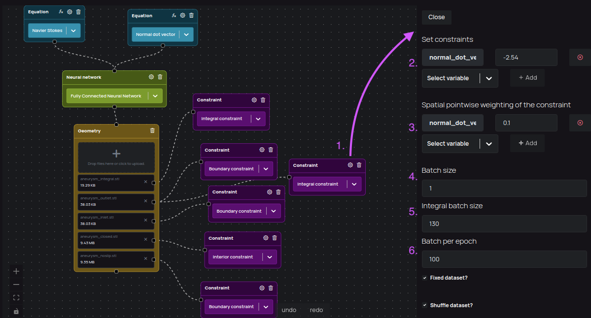
Figure 2.: Constraint settings, accessible by clicking on the "cog" icon after you select a constraint type.
Customizing a constraint node
1. Accessing constraint settings
To access and set constraint settings, you first need to select the type of the constraint node in the visual editor. Then, click on the "cog" icon and right panel with the settings will show up.
2. Setting the constraint's output variables
The outvar parameter is used for describing the constraint. The outvar dictionaries are used when unrolling the computational graph and computing the loss. The number of points to sample on each boundary are specified using the Batch size parameter.
It is often advantageous to work with the nondimensionalized form of physical quantities and PDEs. This can be achieved by output scaling, or nondimensionalizing the PDEs itself using some characteristic dimensions and properties. Simple tricks like these can help improve the convergence behavior and can also give more accurate results.
Figure 3.: Set non-dimensionalized physics constraint on the variables
available in the computational graph from equation nodes. Vlue of the u and
v output is 0.0 on that boundary, and the value of the w output is 1.5 on
that boundary (when dealing with velocity, w often describes velocity along
Z-axis).
3. Setting the constraint's loss function spatial weighting
One area of considerable interest is weighting the losses with respect to each other. The choice for the weighting can be varied based on problem definition, and this is an active field of research. In general, it is beneficial to weight losses lower on sharp gradients or discontinuous areas of the domain. For example, if there are discontinuities in the boundary conditions, we may have the loss decay to 0 on these discontinuities.
Another example is weighting the equation residuals by the signed distance function, SDF, of the geometries, by using a Symbol from sympy, and defining this weighting as Symbol("sdf"). If the geometry has sharp corners, this often results in sharp gradients in the solution of the differential equation. Weighting by the SDF tends to weight these sharp gradients lower and often results in a convergence speed increase and sometimes also improved accuracy.
Figure 4.: Set pointwise weighting for the constraint on the variables available in the computational graph from equation nodes.
4. Batch size
The constraint's Batch size field specifies the number of points to sample on each boundary from connected geometry.
5. Integral batch size for Integral constraint type
In integral constraint, Batch size works differently. It will randomly generate samples that can be controlled by Batch size number, and the points in each sample can be configured with Integral batch size field.
6. Batch per epoch
If Fixed dataset is checked, then the total number of integrals generated to apply constraint on is Total number of integrals = Batch per epoch * Batch size.